Case Studies

Assessing Foundation Conditions and Ground Instability

Detecting subsurface voids with GPR

Lai et al. (2018) showed that 200 MHz GPR can reliably detect air-filled voids as small as 0.4 m in diameter at depths of up to 1.6 m below reinforced concrete (Fig. 1). The voids were built into a 10x20m² test site using air-filled exercise balls. Pipes were added to complicate detection. GPR reliably located four of six voids as shown by the blackened circles in Fig. 2. If there is not a significant amount of clay or conductive water at the site, GPR is the preferred technique because of the significant permittivity contrast between air, water, and fill as well as high spatial resolution and rapid data acquisition.

Fig. 1. Map of test site showing locations of six voids (colored circles) built into the site as well as pipes (green and brown lines). The voids are air-filled exercise balls. Listed at right are depths to void centroids (S= 0.62-1 m) and void diameters (D: 0.4 – 1.6 m). The green lines represent 3 PVC pipes of 50 mm diameter at a depth of 0.85 m. Brown lines represent 1 iron pipe with a diameter of 0.2 m at a depth of 0.66 m. The site was backfilled with sand and covered with concrete (x-axis: 0-10 m) and paving block (x-axis:10-20 m).

Fig. 2. Map of voids detected by GPR (black circles) using a 200 MHz antenna and actual voids from Fig. 1. Four out of six voids were closely located with GPR.  The two other voids (7and 8) were recognized but the estimated and observed locations differed by ~ 1 m.  Brown and green lines as in Fig. 1.

Estimating soil water content over time from ERI to diagnose slope instability

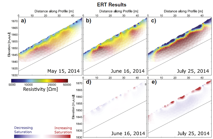
Lucas et al. 2017 collected ERI profiles over a 50 m length of an alpine slope at several times of the year and separately measured rainfall and soil water content (Fig. 3). They show that volumetric water content in gravelly soils is well estimated using ERI and Archie’s Law. ERI also provides much of the ground model (depth to bedrock, soil inhomogeneity) used for modeling of slope instability.  

Fig. 3. a-c) ERI resistivity distribution on an alpine slope on 3 days of increasing wetness. On and just before May 15, 2014, the ground was relatively dry. On and just before July 25, the ground was relatively wet. Note how the resistivity of the soil significantly decreased on 7/25/2014 relative to 5/14/2014 (bluer). The bedrock surface is the top of the highly resistive (red) zone. d-e) ERI interpretation in terms of changes in water saturation relative to 5/14/2014 calculated using Archie’s law and other parameters measured in the field. ERI data indicates that the soil layer contains more water in July than in May, critical information for slope assessment.